Loop Exercise

Exercise 1

Create a dataframe from the “Datasaurus.tsv” file with the following code:

data <- read.csv(
    paste0(
        "https://raw.githubusercontent.com/",
        "nickeubank/computational_methods_boot_camp/",
        "main/source/data/Datasaurus.tsv"
    ),
    sep = "\t"
)

Datasaurus.tsv is a tab-separated-value file, so it’s like a CSV, but it uses tabs not commas to separate columns. We can read this with read.csv, but we have to tell it that the column separator is a tab with the argument sep="\t". Take a look at a few of the top rows:

head(data)

A data.frame: 6 x 26

	example1_x	example1_y	example2_x	example2_y	example3_x	example3_y	example4_x	example4_y	example5_x	example5_y	...	example9_x	example9_y	example10_x	example10_y	example11_x	example11_y	example12_x	example12_y	example13_x	example13_y
	<dbl>	<dbl>	<dbl>	<dbl>	<dbl>	<dbl>	<dbl>	<dbl>	<dbl>	<dbl>	...	<dbl>	<dbl>	<dbl>	<dbl>	<dbl>	<dbl>	<dbl>	<dbl>	<dbl>	<dbl>
1	32.33111	61.41110	51.20389	83.33978	55.99303	79.27726	55.3846	97.1795	51.14792	90.86741	...	47.69520	95.24119	58.21361	91.88189	50.48151	93.22270	65.81554	95.58837	38.33776	92.47272
2	53.42146	26.18688	58.97447	85.49982	50.03225	79.01307	51.5385	96.0256	50.51713	89.10239	...	44.60998	93.07584	58.19605	92.21499	50.28241	97.60998	65.67227	91.93340	35.75187	94.11677
3	63.92020	30.83219	51.87207	85.82974	51.28846	82.43594	46.1538	94.4872	50.20748	85.46005	...	43.85638	94.08587	58.71823	90.31053	50.18670	99.69468	39.00272	92.26184	32.76722	88.51829
4	70.28951	82.53365	48.17993	85.04512	51.17054	79.16529	42.8205	91.4103	50.06948	83.05767	...	41.57893	90.30357	57.27837	89.90761	50.32691	90.02205	37.79530	93.53246	33.72961	88.62227
5	34.11883	45.73455	41.68320	84.01794	44.37791	78.16463	40.7692	88.3333	50.56285	82.93782	...	49.17742	96.61053	58.08202	92.00815	50.45621	89.98741	35.51390	89.59919	37.23825	83.72493
6	67.67072	37.11095	37.89042	82.56749	45.01027	77.88086	38.7179	84.8718	50.28853	82.97525	...	42.65225	90.56064	57.48945	88.08529	30.46485	82.08923	39.21945	83.54348	36.02720	82.04078

Exercise 2

This dataset actually contains 13 separate example datasets, each with two variables named example[number]_x and example[number]_y.

In order to get a better sense of what these datasets look like, our first goal will be to write a loop that iterates over each example dataset (numbered 1 to 13) and prints out the mean and standard deviation for example[number]_x and example[number]_y for each dataset.

For example, the first iteration of this loop might return something like (note I’m also rounding my answers for readability):

Example Dataset 1:
Mean x: 23.123,
Mean y: 98.242,
Std Dev x: 21.247,
Std Dev y: 32.243,
Correlation: -0.742

(Though you shouldn’t get those specific values)

But as we discussed in our reading, we want to approach this in stages. So first, write out the skeleton of your loop. Don’t put anything in it except to print out the value of the variable that is iterating in the loop for now.

Note: the function in R for the correlation between two variables may not be what you think it is…

Exercise 3

Now sketch out what the inside of your loop will look like. As discussed in the readings, begin by creating a variable that takes on the first value you’ll loop over, then, using that variable, write code that does what you want your first pass of the loop to do.

You’ll probably need to make use of print(), paste0(), and round().

Round your answers to three decimal places. Note these numbers should look very similar across datasets.

Exercise 4

Now put them together! Can you print out these summary statistics for all 13 pairs of variables?

Exercise 5

Based only on these results, discuss what might you conclude about these example datasets with your partner. Write down your thoughts.

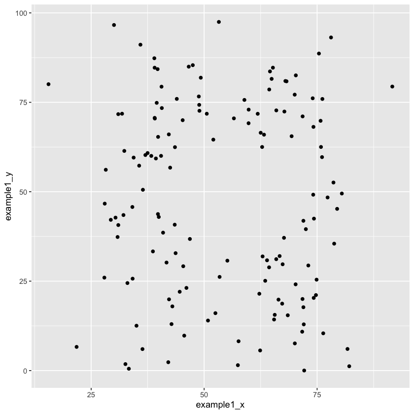
Exercise 6

Now we’re going to write a loop that plots these datasets out in a scatter plot. To do this, we’ll be using the library ggplot2, a libraries from the tidyverse the is unequivocally the best tool for plotting in R.

We aren’t going to do a full lesson on ggplot because you’re sure to encounter it in the future, but the basic syntax to plot the first dataset would look like this:

library(ggplot2)

# First is the dataset, then within `aes_string()` you specify
# which column from the data is the x-axis and which column is the y-axis,
# then `+ geom_point()` tells ggplot to plot points for each line of the data.

ggplot(data, aes(x = .data[["example1_x"]], y = .data[["example1_y"]])) +
    geom_point()

Now build a loop that plots a scatter plot of all 13 of these data pairs. As before, approach it first by writing a skeleton loop that specifies how the loop will work, then write the inside separately, then integrate the two.

Note: if you’ve used ggplot before, note that we’re passing the name of our variables ("example1_x") as a string inside .data[[]]—this avoids the tidyverse odd evaluation problem so you can pass characters as text in double quotes and variables as text not in quotes like normal!

Note: your ggplot may only show up if you wrap it in a print() when it’s inside your loop!

Exercise 7

Review you plots. How does your impression of how these datasets differ from what you wrote down in Exercise 3?

Solutions

Here’s the deal with programming: the only way to learn to program is to wrestle with solving your own problems. The best way to learn is to do so actively – if you just look at answers as soon as you get stuck, your process is more passive. You may feel like you’re learning more, but research shows that that’s an illusion – students who learn passively think they’re learning more than they are (a summary of work in this area is here).

Moreover, in coding in particular, the process of debugging your code is a critical skill in and of itself, and the only way you will learn to do it is by literally spending hours working through your own problems. And once you’ve seen an answer, there’s no way to unsee it, so proceed only if you absolutely have to.

OK, if you still want to proceed, you can find solutions here.