Manipulating Vectors
In our last reading, we learned what vectors were, and how to do operations on entire vectors. But often times we want to work with subsets of a vector. Indeed, extracting a subset of elements from a vector is an extremely important task, not least because it generalizes nicely to datasets (which are at the heart of data science). This process — whether applied to a vector or a dataset — is often referred to as “taking a subset,” “subsetting,” “querying,” or “filtering”. If there is one skill you need to master as quickly as possible, it’s this.
Subsetting can be accomplished in three ways:
By index
By logical vectors (remember I said logicals would be important? :))
By name
What is Subsetting?
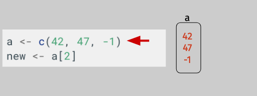
As you’ve probably already realized, vectors don’t just contain a jumble of data – they also have a concept of “order”. When I create a vector with c(42, 47, -1), I have in mind that 42 is the first entry, 47 is the second, and -1 is the third. And we can use that concept of order to subset vectors by passing the index (order number) of an entry we want to our vector in square brackets. For example, consider the following vector:
[1]:
a <- c(42, 47, -1)
a
- 42
- 47
- -1
If I wanted to pull out the second entry in that vector, I could do so with array indexing using square brackets ([]):
[2]:
a[2]
And of course, if I wanted to assign that second entry to a new variable, I could!
[3]:
new <- a[2]
new
But what, exactly, is happening when I subset? Let’s return to the idea that a variable is just a box holding some data, and walk-through the following block of code:
a <- c(42, 47, -1)
new <- a[2]
In the first line of code, we create a new vector with three entries and assign it to the variable a. Just as in our previous reading, we can think of the variable a as a box that is holding this new vector.
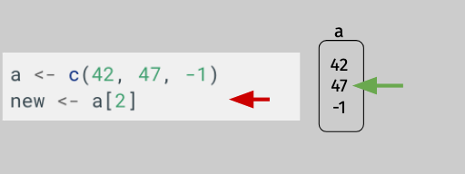
In the second line, the first thing that happens is R evaluates the expression on the right side of the assignment operator: a[2]. The use of a and square brackets indicates to R that we’re not trying to access a portion of the data stored in the box labelled a. In particular, by putting a 2 between the square brackets, we’re telling R we want the second item in the box a: 47.
Then when we assign that value – 47 – to new, we create a new variable, and insert our data into that box:
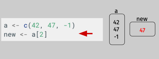
This variable[] notation is something we’ll use a lot in R, and it will always mean the same thing: we’re trying to access some data in the data stored in the box variable.
Subsetting By Index
What we just did is an example of subsetting by index, where we just specify the location (index) of the data we want:
[4]:
a <- c(42, 47, -1)
a[2]
But of course, because everything in R is a vector, if I can pass a single index, then I can pass any other numeric vector of indices, either directly:
[5]:
a[c(1, 3)]
- 42
- -1
Or as a variable:
[6]:
subset <- c(1, 3)
a[subset]
- 42
- -1
Also, you don’t have to subset entries in order! If you pass indices out of order, you’ll get a vector with a new order!
[7]:
a[c(3, 1)]
- -1
- 42
Again, this is all working the same was as our example with just one entry – R interprets the square brackets as a request for some data in the box a, and if we pass multiple indices, it just grabs multiple items from that box.
Subsetting with Logicals
Subsetting with logicals is a little hard to explain, so instead let’s jump right into an example.
Suppose we have a character vector with only two elements (“apple” and “banana”). Subsetting it to “apple” could be done by passing a logical vector as follows:
[8]:
fruits <- c("apple", "banana")
fruits[c(TRUE, FALSE)]
Within these brackets is a vector with the same number of logical elements as there are elements in the vector you want to subset. Elements across the two vectors are matched by order: elements that match with TRUE are kept while elements that match with FALSE are dropped.
Visualized with the same tools we used before, we can draw out what’s happening in this block of code:
[9]:
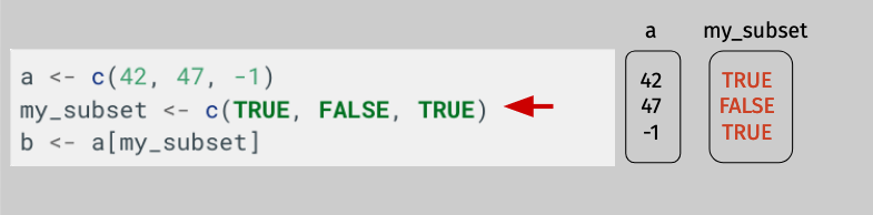
a <- c(42, 47, -1)
my_subset <- c(TRUE, FALSE, TRUE)
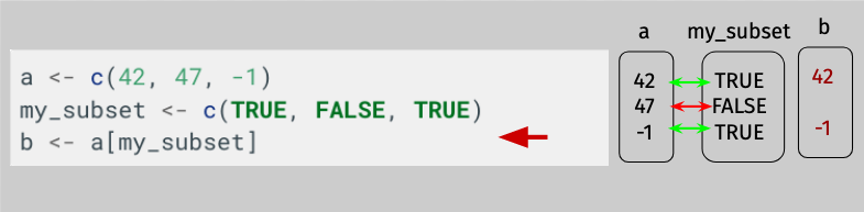
b <- a[my_subset]
b
- 42
- -1
First we create a:
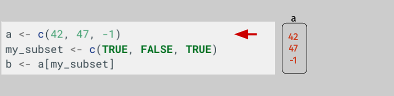
Then we create my_subset:
Then the magic: R lines up the entries in the data in the box labelled a and the data in the box labelled my_subset, and keeps any entries from a that line up with values of my_subset that are TRUE.
Then it assigns the values in a that line up with TRUEs in my_subset to a new variable b:
Logical Operations
This process is extremely useful when combined with a logical operation to combine multiple conditions. For example, you can use:
the logical “and” (written
&in R) to say “only be true if both conditions are true”,the logical “or” (written
|) to say “be true if at least one of these conditions is true”,the logical “equals” (written
==) to say “be true if values are equal”,the logical “not equals (written
!=) to say “be true if values are not equal”, orthe logical “not” (written
!) to say “make everything the opposite of what it is now”.
For example, using a logical operation we can filter a large vector of oranges, apples and bananas:
[10]:
# Create a vector with 30 fruits
fruits <- rep(c("orange", "apple", "banana"), 10)
fruits
- 'orange'
- 'apple'
- 'banana'
- 'orange'
- 'apple'
- 'banana'
- 'orange'
- 'apple'
- 'banana'
- 'orange'
- 'apple'
- 'banana'
- 'orange'
- 'apple'
- 'banana'
- 'orange'
- 'apple'
- 'banana'
- 'orange'
- 'apple'
- 'banana'
- 'orange'
- 'apple'
- 'banana'
- 'orange'
- 'apple'
- 'banana'
- 'orange'
- 'apple'
- 'banana'
[11]:
# Create a logical vector for dropping bananas

orange_or_apple <- fruits == "orange" | fruits == "apple" # TRUE if orange OR apple
not_banana <- fruits != "banana" # TRUE if not equal
not_banana2 <- !(fruits == "banana") # Also TRUE if not equal

# Carry out the subset
fruits[orange_or_apple]
- 'orange'
- 'apple'
- 'orange'
- 'apple'
- 'orange'
- 'apple'
- 'orange'
- 'apple'
- 'orange'
- 'apple'
- 'orange'
- 'apple'
- 'orange'
- 'apple'
- 'orange'
- 'apple'
- 'orange'
- 'apple'
- 'orange'
- 'apple'
[12]:
fruits[not_banana]
- 'orange'
- 'apple'
- 'orange'
- 'apple'
- 'orange'
- 'apple'
- 'orange'
- 'apple'
- 'orange'
- 'apple'
- 'orange'
- 'apple'
- 'orange'
- 'apple'
- 'orange'
- 'apple'
- 'orange'
- 'apple'
- 'orange'
- 'apple'
[13]:
fruits[not_banana2]
- 'orange'
- 'apple'
- 'orange'
- 'apple'
- 'orange'
- 'apple'
- 'orange'
- 'apple'
- 'orange'
- 'apple'
- 'orange'
- 'apple'
- 'orange'
- 'apple'
- 'orange'
- 'apple'
- 'orange'
- 'apple'
- 'orange'
- 'apple'
We applied the same logic as above: We have a vector (fruits) that we want to subset. We do so using a logical vector (orange_or_apple, not_banana, and orange_or_apple2), where elements that match with TRUE are kept. The only difference here is that we create the logical vector with a logical operation. The logical operators (e.g., !=, |) used here are discussed in the link above.
In addition, we can also use the %in% operator as follows:
[14]:
orange_or_apple2 <- fruits %in% c("orange", "apple")
fruits[orange_or_apple2]
- 'orange'
- 'apple'
- 'orange'
- 'apple'
- 'orange'
- 'apple'
- 'orange'
- 'apple'
- 'orange'
- 'apple'
- 'orange'
- 'apple'
- 'orange'
- 'apple'
- 'orange'
- 'apple'
- 'orange'
- 'apple'
- 'orange'
- 'apple'
General note about %in%: This operator is extremely useful as an alternative for repeated “or” (|) statements. For example, say you have a vector with 10 types of fruits and you want to keep elements that are equal to “orange”, “apple”, “mango”, “mandarin”, or “kiwi”. You could accomplish this by creating a logical vector like so: lv <- fruits == "orange" | fruits == "apple" | fruits == "mango" | fruits == "mandarin" | fruits == "kiwi".
What a nighmarishly long statement compared to the %in% option that accomplishes the exact same thing: lv <- fruits %in% c("orange", "apple", "mango", "mandarin", "kiwi").
Of course, subsetting using logicals can also be done on numeric vectors.
Here are a few examples:
[15]:
# Create a numeric vector
numbers <- seq(0, 100, by = 10)
numbers
- 0
- 10
- 20
- 30
- 40
- 50
- 60
- 70
- 80
- 90
- 100
[16]:
# Illustrate three different filters
numbers[numbers <= 50 & numbers != 30]
- 0
- 10
- 20
- 40
- 50
[17]:
numbers[numbers == 0 | numbers == 100]
- 0
- 100
[18]:
numbers[numbers > 100] # returns an empty vector
Subsetting by Name
In R, it’s also possible to assign names to entries in a vector, then use those names to subset entries. To illustrate, let me tell you about the zoo I wished I owned. It’s a small zoo, but a happy one, and here was our imagined attendance last week:
Day of Week | Attendees |
|---|---|
Monday | 132 people |
Tuesday | 94 people |
Wednesday | 112 people |
Thursday | 84 people |
Friday | 254 people |
Saturday | 322 people |
Sunday | 472 people |
I can now represent this as a vector by putting attendance in the vector, and then labeling entries by the day of the week:
[19]:
attendance <- c(132, 94, 112, 84, 254, 322, 472)
attendance
- 132
- 94
- 112
- 84
- 254
- 322
- 472
[20]:
names(attendance) <- c(
    "Monday", "Tuesday",
    "Wednesday", "Thursday", "Friday",
    "Saturday", "Sunday"
)
attendance
- Monday
- 132
- Tuesday
- 94
- Wednesday
- 112
- Thursday
- 84
- Friday
- 254
- Saturday
- 322
- Sunday
- 472
Now if I wanted to just get attendance from the weekend I could subset with a vector of names:
[21]:
attendance[c("Saturday", "Sunday")]
- Saturday
- 322
- Sunday
- 472
Using Subsetting to Modifying Vectors
The subsetting logic from above isn’t just for extracting subsets of vectors to analyze – it’s also useful for modifying vectors. The idea here is that instead of keeping elements that meet a logical condition or occur at a specific index, we can change them. For example, what if we had mis-entered grandpa’s age above? We can fix it using indexing, a logical statement, or naming.
[22]:
# Recreate vector with age values
age <- c(50, 55, 80)

# Three ways of changing grandpa's age
# Note: you'd only need to use one of these
age[age == 80] <- 82 # using a logical statement
age[2] <- 45 # using indexing
age
- 50
- 45
- 82
A logical statement is most efficient when we need to change a lot of elements.
[23]:
fruits <- rep(c("orange", "apple", "bamama"), 5)
fruits # bamamas anyone?
- 'orange'
- 'apple'
- 'bamama'
- 'orange'
- 'apple'
- 'bamama'
- 'orange'
- 'apple'
- 'bamama'
- 'orange'
- 'apple'
- 'bamama'
- 'orange'
- 'apple'
- 'bamama'
[24]:
# Let's fix the misspelled element
fruits[fruits == "bamama"] <- "banana"
fruits
- 'orange'
- 'apple'
- 'banana'
- 'orange'
- 'apple'
- 'banana'
- 'orange'
- 'apple'
- 'banana'
- 'orange'
- 'apple'
- 'banana'
- 'orange'
- 'apple'
- 'banana'
Conditionally Modifying a Subset
The final way that one can use subsets to modify a vector is in a situation where the modification you want to make depends on the value of an observation.
For example, suppose you have the following salary data:
[25]:
salaries <- c(105000, 50000, 55000, 80000, 70000)
salaries
- 105000
- 50000
- 55000
- 80000
- 70000
Now you want to give everyone with an income below $75,000 a $10,000 tax refund. You can’t just do salaries + 10000, because that would apply to all salaries.
One way to address this would be to do it in a couple steps. Create a vector of refund:
[26]:
refund <- replicate(length(salaries), 0)
refund[salaries < 75000] <- 10000
refund
- 0
- 10000
- 10000
- 0
- 10000
[27]:
salaries + refund
- 105000
- 60000
- 65000
- 80000
- 80000
But you can also apply this more directly by subsetting on either side of the assignment operator:
[28]:
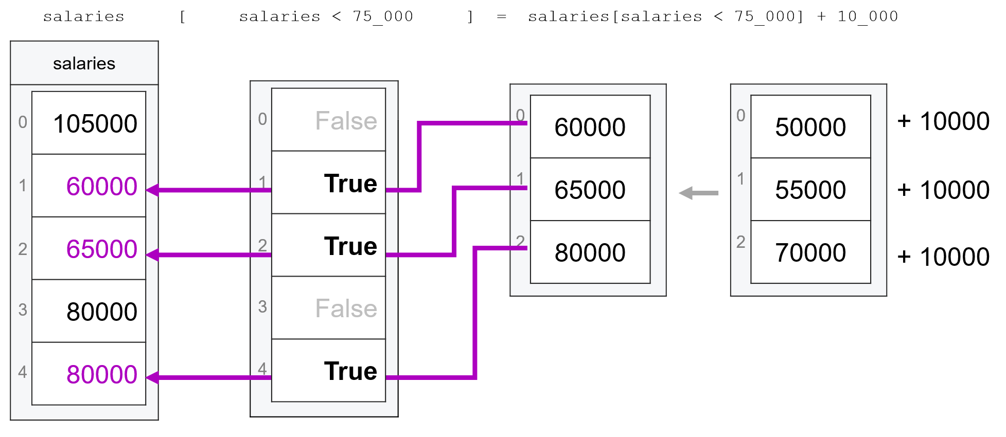
salaries[salaries < 75000] <- salaries[salaries < 75000] + 10000
This can seem very unintuitive at first — the expression on the right hand side of the assignment operator (salaries[salaries < 75000] + 10000) is creating a vector that only has three entries. But salaries has five entries, so where will those three values be assigned?
The answer is that the subsetting on the left-hand-side of the assignment operator ([salaries < 75000]) tells R which entries of salaries are “open” to assignment of new values, as shown in the figure below (sorry about the underscores in the numbers — the figure is originally from Python code, which allows underscores in numbers.)
Recap
Vectors can be subset by index, with a logical, or by name
Subsetting with logicals allows you to extract subsets based on the values of vector elements.
Assigning values to subsets modifies subsets of vectors.
Exercises for Now
Want to practice these skills? Head on over to this site to find some exercises you can do right now!
Exercises for Class
Here are some exercises we’ll be doing in class. Please do not do these before class! If you’re reading these materials on your own or are catching up, feel free to take a look now.